Air Pollution and UV Data Merge

Data Sources

For the climate data we were interested in metrics that were potential risk factors for asthma, lung cancer, and skin cancer, keeping in mind spatial parameters of obtaining data from different states at the county and state level while also looking at longitudinal data across multiple year.

We were able to use a national database maintained by the EPA to obtain daily concentrations of 2 specific air pollutants – inhalable particles termed fine particulate matter (PM_2.5), and ozone gas (O₃) – at the county level across the states from 2001 to 2016. The dataset has no missing values since the it is partially supported by a credible simulation model.

Similar to the air pollution data, we have daily UV measurements at the county level across the states from 2004 to 2015. However, there is occasional missing data and as a result, we ruled out the years populated with missing values for analysis.

For more information about the original data set and methods, see the relevant sites:

Once we imported each of these data sets into R, the data sets were merged across the three states for both longitudinal and cross-sectional data. The data import and cleaning of the original data for UV irradiance, PM_2.5, and ozone can be found in our github repository.

Data Prep

Load packages.

library(tidyverse)
library(rvest)
library(httr)

Scrape FIPS data and put it in a dataframe. See USDA County FIPS.

usda_countyfips = read_html("https://www.nrcs.usda.gov/wps/portal/nrcs/detail/national/home/?cid=nrcs143_013697")

countyfips_string =
  usda_countyfips %>%
  html_elements(".data") %>%
  html_text2()

countyfips_matrix = 
  matrix(
    data = unlist(strsplit(countyfips_string, split = "\r "))[-c(1:3)],
    ncol = 3, 
    byrow = TRUE
  )

countyfips_df =
  tibble(
    countyfips = countyfips_matrix[,1],
    county = countyfips_matrix[,2]
  ) %>%
  mutate(
    countyfips = as.numeric(countyfips)
  )

Load and tidy air pollution data.

pm_df = 
  read_csv("../final_raw/Daily_PM2.5_Concentrations_All_County__2001-2016.csv") %>% 
  filter(statefips %in% c(36, 39, 23, 42)) %>% 
  janitor::clean_names() %>% 
  mutate(
    countyfips = statefips*1000 + countyfips,
    day = str_extract(date, "^\\d{2}"),
    day = factor(as.numeric(day)),
    month = str_extract(date, "[A-Z]{3}"),
    month = factor(month)
  )

oz_df = 
  read_csv("../final_raw/Daily_County-Level_Ozone_Concentrations__2001-2016.csv") %>% 
  filter(statefips %in% c(36, 39, 23, 42)) %>% 
  janitor::clean_names() %>% 
  mutate(
    countyfips = as.numeric(statefips)*1000 + countyfips,
    month = factor(month),
    day = factor(day)
  )

Load and tidy UV irradiance data.

uv_df = 
  read_csv("./data/Population-Weighted_Ultraviolet_Irradiance__2004-2015.csv") %>%
  filter(statefips %in% c(36, 39, 23, 42)) %>% 
  mutate(
    day = factor(as.numeric(day)),
    month = factor(month),
    month = recode_factor(month, `1` = "JAN", `2` = "FEB", `3` = "MAR", `4` = "APR",
                          `5` = "MAY", `6` = "JUN", `7` = "JUL", `8` = "AUG",
                          `9` = "SEP", `10` = "OCT", `11` = "NOV", `12` = "DEC", .default = "Other")
  )

Join the air pollution and UV data sensibly, and match the county names using the FIPS dataframe.

ap_uv_df = 
  full_join(pm_df, oz_df, by = c("year", "countyfips", "month", "day")) %>% 
  full_join(., uv_df, by = c("year", "countyfips", "month", "day")) %>% 
  left_join(., countyfips_df, by = "countyfips") %>% 
  mutate(
    statefips = str_extract(countyfips, "^\\d{2}"),
    state = case_when(
      statefips == 36 ~ "NY",
      statefips == 39 ~ "OH",
      statefips == 23 ~ "ME",
      statefips == 42 ~ "PA"
    ),
    year = factor(year),
    state = factor(state),
    state = fct_relevel(state, "ME", "NY", "PA", "OH"),
    countyfips = factor(countyfips),
  ) %>% 
  select(-contains("statefips"), -date) %>% 
  select(year, month, day, countyfips, county, state, everything())

Export the large tidied dataframe whole and its summaries for our project.

tidy_df =
  ap_uv_df %>% 
  mutate(
    season = case_when(
      month %in% (c("MAR", "APR", "MAY")) ~ "Spring",
      month %in% (c("JUN", "JUL", "AUG")) ~ "Summer",
      month %in% (c("SEP", "OCT", "NOV")) ~ "Fall",
      month %in% (c("DEC", "JAN", "FEB")) ~ "Winter"
    ), 
    season = factor(season),
    season = fct_relevel(season, "Spring", "Summer", "Fall", "Winter")
  ) %>% 
  filter(year %in% c(2005:2015)) %>% 
  group_by(year, countyfips, county, state, season) %>%
  summarize(across(pm25_max_pred:i380, median, na.rm = TRUE), 
            across(pm25_max_pred:i380, round, 2)) %>% 
  ungroup()

saveRDS(tidy_df,"ap/apuv_map/apuv.RDS")

extreme_value =
  bind_cols(
    tidy_df %>% 
      select(pm25_med_pred, o3_med_pred, edd)%>%
      summarize(across(pm25_med_pred:edd, max, na.rm =TRUE))
  ) %>%
  bind_cols(
    tidy_df %>%
      select(pm25_med_pred, o3_med_pred, edd) %>%
      summarize(across(pm25_med_pred:edd, min, na.rm =TRUE))
  )

saveRDS(extreme_value,"ap/apuv_map/ext_val.RDS")

A snippet of the resulting data set:

library(kableExtra)

knitr::opts_chunk$set(
    fig.asp = 0.75,
    fig.width = 6,
    message = FALSE,
    warning = FALSE,
    out.width = "100%"
)

tidy_df <-
  read_csv("./ap/ap_uv/apuv.csv") %>% 
  janitor::clean_names() %>% 
  filter(year == 2005, state == "NY")

kbl(tidy_df[1:7,]) %>% 
  kable_styling(bootstrap_options = c("striped", "hover"), full_width = T) %>% 
  scroll_box(width = "100%", height = "200px")

year	countyfips	county	state	season	pm25_max_pred	pm25_med_pred	pm25_mean_pred	pm25_pop_pred	o3_max_pred	o3_med_pred	o3_mean_pred	o3_pop_pred	edd	edr	i305	i310	i324	i380
2005	36001	Albany	NY	Fall	8.46	8.17	8.02	8.07	33.11	29.21	29.56	29.57	1123.23	64.03	14.66	32.94	176.72	342.32
2005	36001	Albany	NY	Spring	9.26	8.84	8.72	8.74	48.76	45.79	46.04	45.98	2069.77	99.02	23.44	51.58	268.05	498.51
2005	36001	Albany	NY	Summer	15.68	15.11	15.02	15.08	49.85	47.98	47.84	47.84	3914.38	175.79	49.98	85.13	331.90	616.02
2005	36001	Albany	NY	Winter	12.79	12.07	12.07	12.14	32.12	27.64	27.88	27.84	429.64	26.08	2.56	11.16	104.63	206.31
2005	36003	Allegany	NY	Fall	8.50	7.30	7.45	7.34	35.61	35.21	35.09	35.08	1135.08	64.24	14.56	32.82	173.15	351.96
2005	36003	Allegany	NY	Spring	8.87	7.95	8.01	7.99	48.71	47.51	47.62	47.61	2059.54	99.84	25.32	52.42	245.47	458.43
2005	36003	Allegany	NY	Summer	14.83	14.14	14.13	14.13	54.38	52.72	52.79	52.76	4045.63	181.38	52.39	88.74	334.92	619.09

Variable Definitions

year. Year
countyfips. County-level unique identifier
county. Name of county
state. 2-character abbreviation of state name
season. Period of year in which data was collected
pm25_max_pred. Daily county-level maximum \(PM_{2.5}\) recorded/simulated, \(\mu g/m^3\)
pm25_med_pred. Daily county-level median \(PM_{2.5}\) recorded/simulated, \(\mu g/m^3\)
pm25_mean_pred. Daily county-level mean \(PM_{2.5}\) recorded/simulated, \(\mu g/m^3\)
pm25_pop_pred. Daily county-level population weighted mean \(PM_{2.5}\) recorded/simulated, \(\mu g/m^3\)
o3_max_pred. Daily county-level maximum \(O_{3}\) recorded/simulated, \(ppm\)
o3_med_pred. Daily county-level median \(O_{3}\) recorded/simulated, \(ppm\)
o3_mean_pred. Daily county-level mean \(O_{3}\) recorded/simulated, \(ppm\)
o3_pop_pred. Daily county-level population weighted mean \(O_{3}\) recorded/simulated, \(ppm\)
edd. Daily county-level population weighted erythemally weighted daily dose, \(J/m^2\)
edr. Daily county-level population weighted erythemally weighted irradiance at local solar noon time, \(mW/m^2\)
i305. Daily county-level population weighted spectral irradiance at local solar noon time at 305 nm, \(mW/m^2/nm\)
i310. Daily county-level population weighted spectral irradiance at local solar noon time at 310 nm, \(mW/m^2/nm\)
i324. Daily county-level population weighted spectral irradiance at local solar noon time at 324 nm, \(mW/m^2/nm\)
i380. Daily county-level population weighted spectral irradiance at local solar noon time at 380 nm, \(mW/m^2/nm\)

Visualizing Trends in Climate Data over Space and Time

knitr::opts_chunk$set(
    fig.asp = 0.75,
    fig.width = 6,
    message = FALSE,
    warning = FALSE,
    out.width = "100%"
)

library(patchwork)
scale_colour_discrete = scale_color_viridis_d
scale_fill_discrete = scale_fill_viridis_d
theme_set(theme_bw() + theme(plot.caption = element_text(size = 6.5)))

# Ozone
o3_time <-
  read_csv("./ap/ap_uv/o3.csv") %>% 
  janitor::clean_names() %>% 
  filter(state == "NY" | state == "OH" | state == "PA") %>% 
  select(-hover) %>% 
  janitor::clean_names() %>% 
  mutate(county = tolower(county))

o3_lreg <-
  o3_time %>% 
  ggplot(aes(x = year, y = o3, color = season)) +
  geom_point(alpha = 0.1) +
  geom_smooth(method = "loess", se = TRUE) +
  labs(x = "Year", y = "Ozone (ppb)", color = "Season") +
  theme(legend.position = "top") +
  facet_grid(. ~ state) 

# PM2.5 plot
pmname = expression(PM~2.5~(µg/cm^2))

pm_time <-
  read_csv("./ap/ap_uv/pm25.csv") %>% 
  janitor::clean_names() %>% 
  filter(state == "NY" | state == "OH" | state == "PA") %>% 
  select(-hover) %>% 
  janitor::clean_names() %>% 
  mutate(county = tolower(county))

pm_lreg <-
  pm_time %>% 
  ggplot(aes(x = year, y = pm2_5, color = season)) +
  geom_point(alpha = 0.1) +
  geom_smooth(method = "loess", se = TRUE) +
  labs(x = "Year", y = pmname) +
  theme(legend.position = "none") +
  facet_grid(. ~ state) 

# UV plot

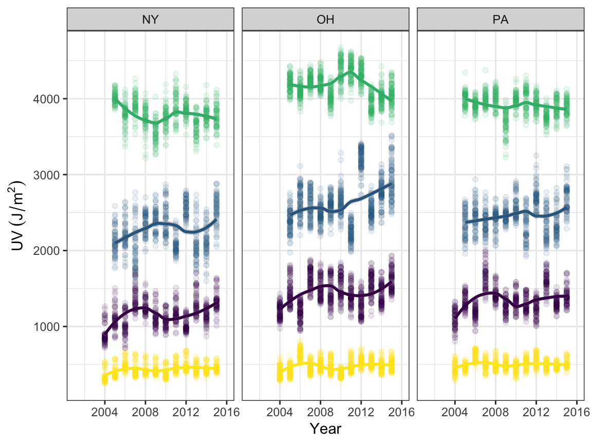
name_uv = expression(UV~(J/m^2))

uv_time <-
  read_csv("./ap/ap_uv/edd.csv") %>% 
  janitor::clean_names() %>% 
  filter(state == "NY" | state == "OH" | state == "PA") %>% 
  select(-hover) %>% 
  mutate(county = tolower(county))

uv_lreg <-
  uv_time %>% 
  ggplot(aes(x = year, y = uv, color = season)) +
  geom_point(alpha = 0.1) +
  geom_smooth(method = "loess", se = TRUE) +
  labs(x = "Year", y = name_uv) +
  theme(legend.position = "none") +
  facet_grid(. ~ state) 

o3_lreg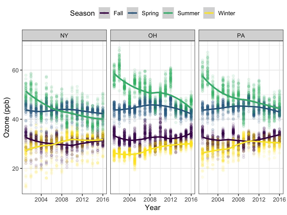

pm_lreg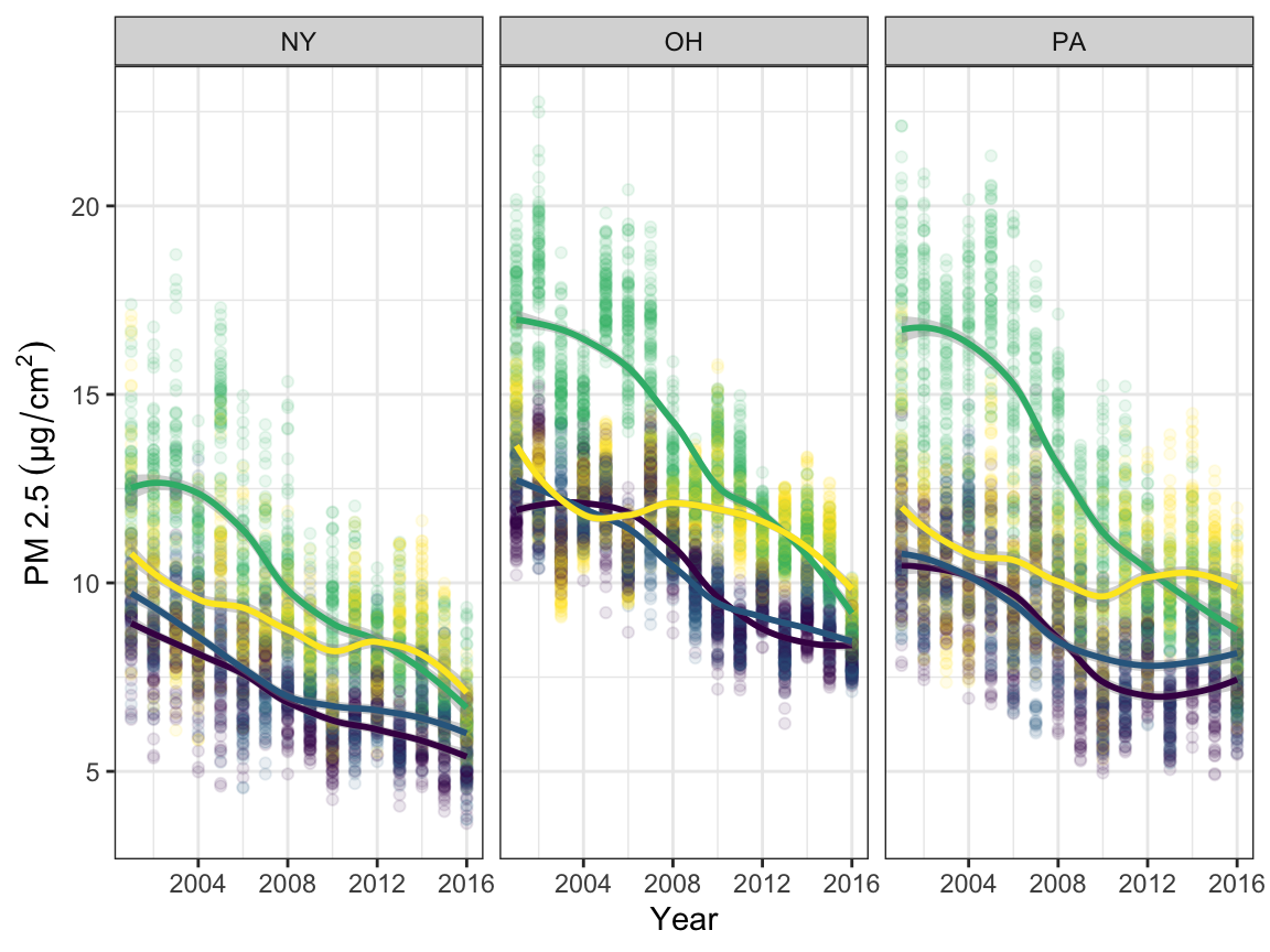

uv_lreg